Deep Learning Meets Gaussian Process: How Deep Kernel Learning Enables Autonomous Microscopy
Maxim Ziatdinov¹ ² & Sergei V. Kalinin¹
¹ Center for Nanophase Materials Sciences and ² Computational Sciences and Engineering Division, Oak Ridge National Laboratory, Oak Ridge, TN 37831, United States
For many scientists and engineers, the road towards their profession started from microscopy. Under a simple optical microscope or a magnifying glass, the sand from the nearby beach starts to look like a mountain country containing skeletons of diatoms and snails and pieces of colorful minerals. The droplet of water from the puddle reveals curious (and sometimes disturbing) microscopic denizens. With modern phones, the Google Lens can help identify their class and genus. The dried salt solution will show rainbow-colored crystals. In a more professional setting, the bespoke (and much more expensive) electron and scanning probe microscopes reveal micron and nanometer-scale structures of the material, going all the way to visualize atomic patterns forming the materials and molecules laying on their surfaces. The figure below shows the golden orb spider imaged by the second author and the “buckyball” molecules on the surface imaged by the first.

Yet the modern microscopes allow not only to image materials and their surfaces but also to perform much more detailed studies of their properties. In scanning tunneling microscopy (STM), the operator can choose potentially interesting regions and perform tunneling spectroscopy, i.e., measure the current-voltage curves. Controlled by quantum tunneling, this curve will contain information about the local density of states, superconductivity, charge density waves, and other exciting phenomena on the surface [1–2]. In electron microscopy, the technique of choice is electron energy loss spectroscopy [3]. Here, measuring the energy loss of electrons passing through the solid reveals the chemical structure of individual atoms and, with recent advances in monochromated instruments, allowed probing quasiparticles such as electrons and plasmons in solids [4–5]. The particularly broad gamut of the possible spectroscopic modes emerged in the scanning probe microscopies, allowing researchers to probe local mechanical properties, conductivity, and ferroelectric polarization switching [6–7].
Unfortunately, the local functional measurements take a lot of time compared to imaging. For example, getting a simple STM image often takes about 5–10 minutes. Getting the dense array of spectroscopic curves over a dense spatial grid of points takes days, necessitating building ultrastable microscopes that will not drift appreciably over these times. The same considerations apply to electron microscopes, for which additional consideration is sample damage by the electron beam. Finally, many measurements are destructive and cannot be taken over the dense grid, for example, nanoindentation. These considerations severely limit the capabilities of these measurements and the insight they provide into the material’s structure and functionality. Much like proverbial Jon Snow, if we do not know where to measure, we measure everywhere hoping to capture the behaviors of interest during the ex-situ data analysis, hoping to identify the regions of interest. Can we do better with machine learning? (hint: we can, otherwise this blog post would not be written).

In order to understand what it takes to make this work, we first consider the paradigmatic approach for active learning in experiments based on Gaussian Process (GP). In most general form, GP refers to the class of algorithms that attempt to reconstruct the function over certain (low dimensional) parameter space from a set of sparse measurements. In other words, given a set of observed data points (xᵢ, yᵢ) and assuming normally distributed observation noise ϵ, the GP aims to reconstruct the function f(x) such as yᵢ= f(xᵢ) + ϵᵢ, with f ~ MultivariateNormal(0; K(xᵢ, xⱼ)). The functional form of the kernel K is chosen prior to the experiment, and its hyperparameters are inferred from the observations using either Markov chain Monte Carlo methods or stochastic variational inference. You can read about the more rigorous definition of GP here. Please see also our previous Medium post on GPs. Our group has applied GP to a number of imaging problems including reconstruction of sparse hyperspectral data, hysteresis loop engineering in ferroelectrics, and efficient exploration of the parameter space for lattice Hamiltonians, and the full codes are available through the GPim package.
The unique aspect of GP is that the function is reconstructed along with the associated uncertainty Σ(x). This aspect allows extending GP towards the active learning methods. Suppose we want to learn the value of the function over parameter space in the most effective way by sequentially selecting points to perform the measurements. In that case, the region with the maximal uncertainty represents the optimum point for a query. In this manner, a GP-driven automated experiment seeks to reduce the uncertainty about function in the most expeditious manner.
It should be noted the GP can be further extended to target specific behavior. In this case, if we have prior knowledge of what values of the function we are looking for, we can combine the expectation and uncertainty in a single acquisition function. The maximum (or minimum) of the acquisition function is then used for the navigation of the parameter space. This approach combining the exploration and exploitation of the parameter space is generally referred to as Bayesian Optimization (BO).
Then the question becomes whether GP/BO can be utilized to enable automated experiments in microscopy. It turns out that it is possible in the case of simple imaging or spectroscopy, but the total gain is relatively small. Indeed, images typically contain multiple features at many different length scales — from large to small. A priori, we do not know what these features are. Correspondingly, GP-based algorithms that try to navigate image space based on single point measurement and discover the associated kernel function get stumbled. Indeed, for known images, the kernel function is roughly equivalent to the correlation function, and this is not a very effective way to represent the image. In principle, one can work with reduced representation of the image achieved through applying either standard multivariate decomposition (PCA, NMF) or autoencoder techniques to image patches. However, there is no guarantee that these reduced representations will be physically meaningful, and they can be frequently dominated by instrumental factors such as drift (in many cases, a domain expert has to separate physical variables from the unphysical ones, which defies the whole point of the automated experiment). Furthermore, decomposition requires the patches to be available in advance — belying the concept of discovery.
The GP-produced gain is further reduced as the microscope’s electronics and mechanics can start to fail if forced to move the probe along the very complex paths. On top of that, the GP usually does not work well to predict complex patterns. All in all, it looks like the GP it is insufficient for automated experiments in microscopy.
Enter the deep kernel learning. To understand how it works, let’s recap what a human operator would do if they looked at the image. Human eyes immediately register the objects of interest. For example, in the STM image of the superconductor in Figure 2, we can instantly notice the regions with bright spots. A qualified human operator would immediately identify these regions as potentially hosting a localized electronic state(s) although its properties will probably depend on the surrounding. Similarly, one can notice multiple regions with stripy contrast which could be indicative of surface reconstruction. There are many of them and it is intuitively obvious that they should have somewhat similar behaviors. So perhaps it is sufficient to perform a spectroscopic measurement in several of them and assume that the observed behaviors are representative. However, there are also regions where a small depression and/or protrusions are embedded into the stripy domains and those regions may contain some additional interesting insights about the physics of this system. The question then becomes whether we can utilize the information contained in the structural images to guide the spectroscopic measurements in an autonomous fashion.
Deep kernel learning (DKL), originally introduced by Andrew Gordon Wilson, can be understood as a hybrid of classical deep neural network (DNN) and GP, as shown in Figure 3. Here, the DNN part serves as a feature extractor that allows reducing the complex high-dimensional features to low-dimensional descriptors on which a standard GP kernel operates. The parameters of DNN and of GP kernel are optimized jointly by performing a gradient ascent on marginal log-likelihood. The DKL output on the new inputs is the expected value and associated uncertainty for the property (or properties, if we are interested in vector-valued functions) of interest. Let’s see how we can harness DKL to run experiments on the electron or scanning probe microscopes.

We are going to show two basic examples where DKL is used to map parts of a material’s structure that maximize a particular physical functionality. To achieve this, the DKL must learn the correlative structure-property relationship(s) in the system. Implementation-wise, the DKL training inputs are small patches of a structural image, and training targets are scalar values associated with some physical functionality derived from spectra measured in the centers of patches (the DKL can also work with vector-valued targets and can even predict the entire spectra, but these will be discussed in a separate post). The goal is to use easy-to-acquire structural data to guide spectroscopic measurements that are typically much more tedious. Hence, the DKL-based automated experiment begins with collecting a structural image, which is split into a set of small patches (one patch per image pixel), followed by the acquisition of several spectroscopic curves in random locations of the image. These sparse observations are used to train a DKL model. Then, a trained DKL model is used to predict a property of interest in every coordinate of the structural image (or, more specifically, for every image patch centered at that coordinate) for which there is no measured spectrum. The predicted mean property value and associated uncertainty are used to derive an acquisition function to sample the next measurement point(s). Once a new measurement is performed, the training data is updated, and the whole process is repeated.
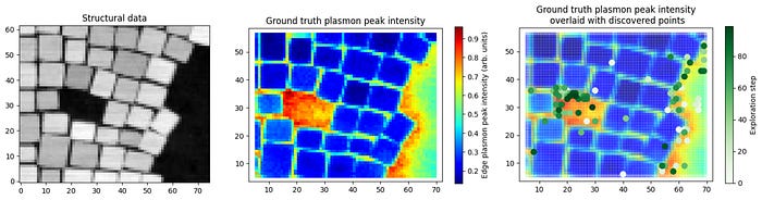
First, let’s use the publicly available dataset obtained on plasmonic nanocubes. Here our structural data come from a scanning transmission electron microscopy image. The functionality of interest is derived from the electron energy loss spectra measured over the same area and, in this particular example, is simply the intensity of the edge plasmon peak. We run DKL for 100 iterations which are about 3% of the total grid points. At each iteration, we select the next measurement point using a simple Thompson sampler. Since we already know the ground truth, we can overlay the sampled points with the ground truth map. One can see that we were able to identify regions within the structural image where the functionality of interest is maximized by measuring only a small fraction of a grid.
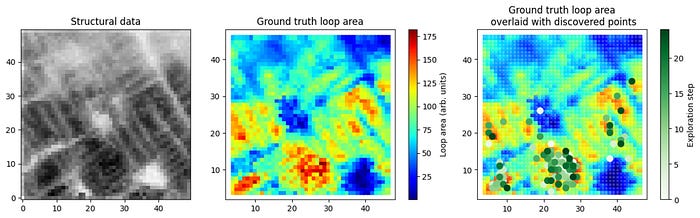
Now, let’s see how this approach works for identifying sample regions that maximize hysteresis loop area in piezoresponse force microscopy. Our DKL setup is almost the same as in the previous experiment, except that now, at each step we sample a batch of 4 points instead of just a single point. Again, as one can see from Figure 5 below, we were able to quickly localize the behavior of interest with a very small number of measurements (~5% of the entire grid).
Overall, this approach uses structural information to guide spectroscopic (functional) measurements by actively learning the structure-property relationships in the system. Importantly, we can use almost any physical search criteria from the simple ones used in this blog post to much more complicated ones. In this manner, we combine the power of correlative machine learning to establish relationships in the multidimensional data set and derive corresponding uncertainties, and domain expertise encoded in the choice of the search criteria.
Please check out our AtomAI software package for applying this and other deep/machine learning tools to scientific imaging. If you want to learn more about the Scanning Probe Microscopy, welcome to channel M*N: Microscopy, Machine Learning, Materials. Finally, in the scientific world, we acknowledge the sponsor that funded this research. This effort was performed and supported at Oak Ridge National Laboratory’s Center for Nanophase Materials Sciences (CNMS), a U.S. Department of Energy, Office of Science User Facility. You can take a virtual walk through it using this link and tell us if you want to know more.
The executable Google Colab notebook for one of the examples is available here.
References:
1. Roushan, P.; Seo, J.; Parker, C. V.; Hor, Y. S.; Hsieh, D.; Qian, D.; Richardella, A.; Hasan, M. Z.; Cava, R. J.; Yazdani, A., Topological surface states protected from backscattering by chiral spin texture. Nature 2009, 460 (7259), 1106-U64.
2. Pan, S. H.; Hudson, E. W.; Lang, K. M.; Eisaki, H.; Uchida, S.; Davis, J. C., Imaging the effects of individual zinc impurity atoms on superconductivity in Bi2Sr2CaCu2O8+delta. Nature 2000, 403 (6771), 746–750.
3. Pennycook, S. J.; Varela, M.; Lupini, A. R.; Oxley, M. P.; Chisholm, M. F., Atomic-resolution spectroscopic imaging: past, present and future. J. Electron Microsc. 2009, 58 (3), 87–97.
4. Kapetanakis, M. D.; Zhou, W.; Oxley, M. P.; Lee, J.; Prange, M. P.; Pennycook, S. J.; Idrobo, J. C.; Pantelides, S. T., Low-loss electron energy loss spectroscopy: An atomic-resolution complement to optical spectroscopies and application to graphene. Phys. Rev. B 2015, 92 (12).
5. Hage, F. S.; Nicholls, R. J.; Yates, J. R.; McCulloch, D. G.; Lovejoy, T. C.; Dellby, N.; Krivanek, O. L.; Refson, K.; Ramasse, Q. M., Nanoscale momentum-resolved vibrational spectroscopy. Sci. Adv. 2018, 4 (6), 6.
6. Kalinin, S. V.; Strelcov, E.; Belianinov, A.; Somnath, S.; Vasudevan, R. K.; Lingerfelt, E. J.; Archibald, R. K.; Chen, C. M.; Proksch, R.; Laanait, N.; Jesse, S., Big, Deep, and Smart Data in Scanning Probe Microscopy. ACS Nano 2016, 10 (10), 9068–9086.
7. Vasudevan, R. K.; Jesse, S.; Kim, Y.; Kumar, A.; Kalinin, S. V., Spectroscopic imaging in piezoresponse force microscopy: New opportunities for studying polarization dynamics in ferroelectrics and multiferroics. MRS Commun. 2012, 2 (3), 61–73.
8. Kalinin, S. V.; Valleti, M.; Vasudevan, R. K.; Ziatdinov, M., Exploration of lattice Hamiltonians for functional and structural discovery via Gaussian process-based exploration-exploitation. J. Appl. Phys. 2020, 128 (16), 11.
9. Kalinin, S. V.; Ziatdinov, M.; Vasudevan, R. K., Guided search for desired functional responses via Bayesian optimization of generative model: Hysteresis loop shape engineering in ferroelectrics. J. Appl. Phys. 2020, 128 (2), 8.

